
Object Detection: where and what
Object Detection comprises two principle aims: finding object locations and recognise the object category (dog or cat), summarised as object localization and classification. Localisation tells the objects from the background while classification tells one object from others with different categories.
one sample image from the faster RCNN paper
Bounding Box and IoU
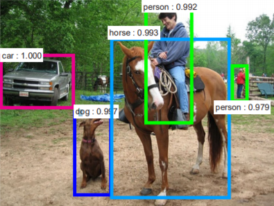
The detection model uses rectangle bounding boxes as its predictions on object location and classification results (as in the demo image below). In other words, the model thought the bounding box contains an object from a certain category.

A demo image of Bounding Boxes
As a supervised machine learning task, both prediction and ground truth are represented as bounding boxes, which is different from the discrete label as image classification tasks such as MNIST. So how to decide the correctness of localisation? Well, the answer is IoU (Intersection of Union), also known as “Jaccard index”, see wiki for the historical details. Adapted from associated conceptions from set theory, IoU is calculated by the division of the areas of intersection and union, as the figures below displaying the areas.
 A demo image of IoU areas
While the formula is given as below:
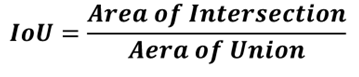
One of the motivations of using is its invariability to bounding box scales,in other words, a high IoU can only be achieved if the predicted bounding box has a close approximation as the benchmark. Besides, It transforms the detection results as simple geometric properties (area, width and height). Regarding the way to decide whether a prediction hits ground truth, a threshold for IoU is pre-defined as proportions marking predictions with a higher IoU (50% (PASCAL VOC), 75% or strict 95%) are considered as the correct predictions.
Also, as the metrics for supervised machine learning, IoU is associated with losses to regress the prediction bounding boxes to the ground truth. [Optional] There is a recent CVPR paper proposed a generalized IoU metric which might make it training easier in some cases.
Precision and Recall
Unlike many computer vision tasks, such as MNIST classification, which uses accuracy to evaluate model performance, Object Detection uses a pairwise metric of precision and recall. These two metrics are originally used in document retrieval then adapted into the machine learning domain. One example is their appliance in image classification, such as classifying whether the image contains a cat or not.
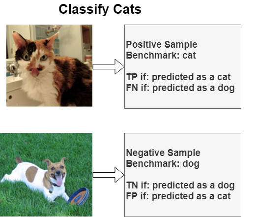
Based on the data sample benchmark, there are four conditions are shown below:
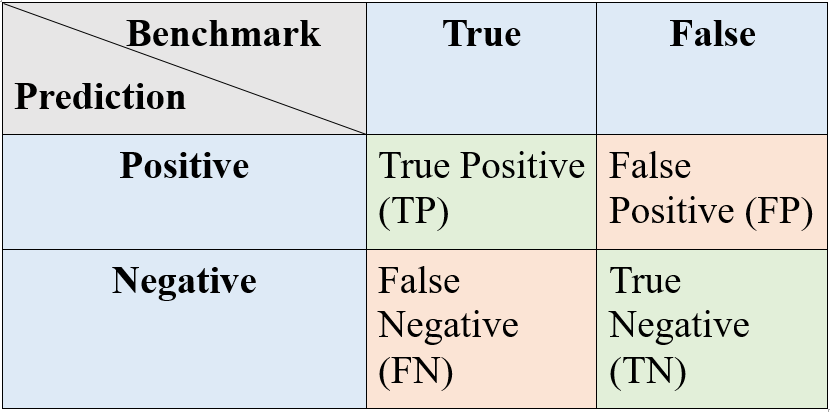
Confusion MatrixTo be specific, for the sample image of cats (benchmark is cat category):
- If the model predicts an image containing a cat, it is denoted as a “positive” prediction making the dog category as “negative”. In this case, the model prediction is correct, which is the “TP” (True Positive) in the table above. For the dog category, this prediction is a correct “TN” (True Negative).
- Similarly, if the model prediction is a dog (Negative for cat and positive for dog), then it is an “FN” (False Negative) for cat and “FP” (False Positive) for the dog.
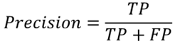
Normally the precision is defined as in the following equation:
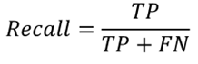
and for recall:
Overall, the addition of TP and FP is considered as the total amount of positive predictions by the model while the sum of TP and FN is the total image amount of the target category in the dataset, i.e. the number of cat images.
In concluding, precision measures the proportion of correctness in the positive predictions which is the likelihood of correctness when the model gives a positive prediction.
While recall reflects the proportion of correctness among all positive data samples, i.e. whether the model predicts most of the instances from the target category.
One of the motivations of applying precision and recall instead of accuracy is its limitation on the imbalanced dataset. In the aspect of the confusion matrix, the metric accuracy is calculated as:
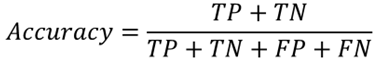
Therefore, accuracy is the proportion of overall correct predictions. It works fine when the dataset has approximately similar instance amounts for each category. However, in practice, it’s commonly the dataset includes categories with more instances than others. For example, the dataset contains 100 images, which comprises 99 cat images and only 1 dog image.
In that case, the high accuracy can be achieved by simply output all images as cats for a 99% accuracy. In other words, the metric of accuracy does not make sense. In contrast, precision for cats is 99% with 100% recall while the dog category is 0% precision with 0% recall. These abnormal precision and recall values indicate the issues in model performance, proving their better usability than accuracy.
From P to AP and P-R curve
The previous section introduces contents on precision, recall and using IoU to evaluate model predictions. Based on these fundamental conceptions, a series of metrics are proposed to describe detailed model performance: P-R curve, AP and mAP.
Regrading the imbalanced dataset example in the previous section, precision or recall itself is not sufficient enough to describe model performance, as precision can be 99% with a 0% recall. Because the precision can be improved simply by outputting a small number of predictions with the highest confidences, such as outputting only one prediction which the model is 100% sure that is a cat to get a 100% precision, as precision is not considering the prediction amount. While a high recall rate can be achieved by increasing prediction amount, such as predicting all data samples as cats to get a 100% recall, since the denominator of recall does not involve the number of false predictions.
Therefore, to include both precision and recall, P-R curve is proposed to systematically describe model precision with different recall levels, as the diagram shown below:
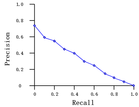
A sample P-R curve
Most P-R curves have the following commonalities:
- It is non-sense when Precision is zero (TP = 0) and approximated values are used instead.
- The “zero recall” is handled similarly. Also, regarding the precision equation, zero recall stands for a large value of “TP + FP” as the prediction amount is largely increased, causing precision converges to zero.
P-R curve describes detailed information on the changes between precision and recall. However, it is not brief enough to summarize model performance and a simple metric is required to compare different models. Therefore the conception of “Average Precision” (AP) is proposed at the early object detection challenge PASCAL VOC, which is adapted from the 11-point interpolation method in the domain of information retrieval. AP is calculated by the equations below:
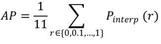
while “r” stands for recall and “P_interp(r)” (oh god, it looks terrible) means the interpolation precision given a recall rate “r”, which is averaged over 11 different recall rate from 0 to 1. The interpolation precision is calculated by the maximum precision the model could reach with recall rates larger than the given “r”. It is a common case that higher recall is associated with lower precision or vice versa.
Therefore the “A” for average in “AP” is the average over the 11 interpolation precisions and in practice, the dataset includes multiple categories and each category has its own AP. Hence, in general, AP also includes extra calculations for the mean value of the category-wise APs.
Besides, Average Recall (AR) is defined and calculated similarly as AP.
So from P to AP, it takes two average calculations: interpolation precisions and computing the category-wise mean. Furthermore, AP demonstrates both precision and recall in a brief way used as the principal metric in PASCAL VOC challenges to determine winners.
From AP/AR to mAP/mAR
As mentioned above, AP summarised precision and recall from the P-R curve and used as main metrics for ranking model performances. However, there are still some unavoidable limits of AP. One of the main limits is its incapacity when most of the candidate models achieved high AP given a loose IoU standard as 0.5. Therefore, mean Average Precision (mAP) is proposed to evaluate model performance given different level of IoU thresholds. Origins from MS-COCO challenge, mAP calculates the mean value of APs given different IoU thresholds.
Regarding the conceptions of IoU in previous sections, lower IoU values stand for lower difficulties that contribute a higher AP. As the development of deep learning models in object detection, model performance has been greatly improved making 0.5 IoU insufficient to rank models.
mAP considers 10 different IoU thresholds and their APs are listed as below:

Besides different IoU thresholds, MS-COCO mAP also specifies model performance on objects with different scales as mAP small, mAP medium and mAP large. The object scales are given by the area of their ground truth bounding boxes (W × H). Objects with scales less than 32×32 pixels are defined as small objects, while the medium ones are those between 32×32 and 96×96 and those greater than 96×96 are considered as large objects.
Therefore, mAP evaluated model performance in a more systematic aspect comparing with AP. mAR is defined and calculated in a similar way and mAP is considered as the principal metric to rank models in MS-COCO challenges.
Object Detection Common Errors and Derek P-R curve
The previous section introduces mAP which evaluates model performance under different recall rate and specified scale related detection outcomes. Besides of mAP, there is another metric called Derek style P-R curve that considers common errors in object detection.
The Derek P-R curve is originally proposed by Derek Hoiem in his paper “Diagnosing Error in Object Detectors” and modified by other researchers to demonstrate detailed model performances.
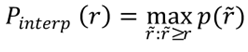
Regarding the aforementioned contents, object detection model predicts bounding boxes to denote object location and classify object category inside the boxes. According to the differences between the predicted bounding box and associated ground truth boxes, the incorrect detection results can be viewed as four different categories: Loc, Sim, Oth and Bg.
- Loc: Loc stands for localisation error which means lower IoU between 10% to 50%.
- Sim: Sim means similar objects error that models incorrectly classified objects as the others within the same super-category such as recognise a bus as a truck while bus and truck belong to the same super-category “vehicle” (a).
- Oth: the detector classifies objects to a category which is from a different super-category such as candle and traffic light (b).
- Bg: the detector classifies part of the background image as an object, such as recognising a background tree as a person (c).
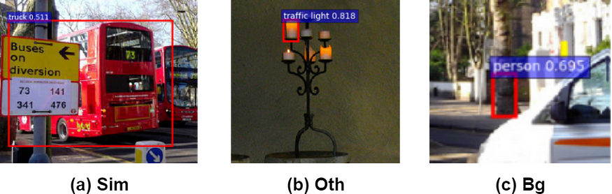
Various reasons are causing these errors such as object scales, the aspect ratio of the ground truth bounding boxes, occlusion and abnormal viewpoints. The below diagram shows an example of aeroplane objects:
The Derek P-R curve is introduced based on the discussion above. The below diagram shows a demon curve of ResNet-50 backboned Faster-RCNN model on the MS-COCO dataset.
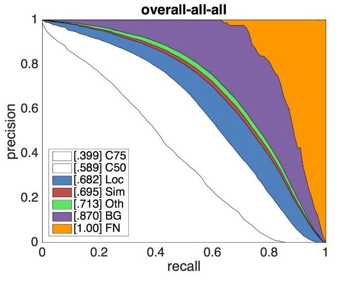
Derek P-R curve demonstrates model performance with its errors by Area Under the Curve (AUC). The areas of different colours denote associated errors and the white part are C75 and C50, which represents model mAP under 75% and 50% IoU thresholds respectively. The Loc boundary curve means the mAP results after tuning IoU threshold from 50% to 10%. Sim, Oth and Bg boundary curves are mAP results after setting associated errors as correctness. Finally, false negative (FN) is used as complementary for the errors that are not included and makes the total area as “1.00”.
References:
- Girshick, R. (2015). Fast r-cnn. In Proceedings of the IEEE international conference on computer vision (pp. 1440–1448).
- Everingham, M., Van Gool, L., Williams, C. K., Winn, J., & Zisserman, A. (2010). The pascal visual object classes (voc) challenge. International journal of computer vision, 88(2), 303–338.
- Lin, T. Y., Maire, M., Belongie, S., Hays, J., Perona, P., Ramanan, D., … & Zitnick, C. L. (2014, September). Microsoft coco: Common objects in context. In European conference on computer vision (pp. 740–755). Springer, Cham.
- Hoiem, D., Chodpathumwan, Y., & Dai, Q. (2012, October). Diagnosing error in object detectors. In European conference on computer vision (pp. 340–353). Springer, Berlin, Heidelberg.
- Manning, C., Raghavan, P., & Schütze, H. (2010). Introduction to information retrieval. Natural Language Engineering, 16(1), 100–103